7 Lead scoring

Suppose I offered you $50,000 to sell four season tickets to someone in the next twenty-four hours. What would you do? The first thing I would ask is what the tickets cost. If it is less than $50,000, I could just buy them myself and pocket the difference. Short of that, how would you raise the odds of selling four real tickets?

• Call a broker and ask them to buy.
• Look for lapsed purchasers.
• Look for abandoned carts on the website.
• Call season-ticket holders who have not yet renewed.
• Beg friends and family.

There are plenty of ways to pick the low-hanging fruit. You would almost never resort to dialing random phone numbers. The question is whether we can make that prioritization analytical instead of intuitive.

That is lead scoring. You can qualify leads many ways, but the goal is always the same: order your leads so your sales effort stays efficient. A warm lead, meaning someone who has engaged with your brand, is worth more of a rep’s time than a cold one. Marketing has been wrestling with this for over a century:

“Half the money I spend on advertising is wasted; the trouble is I don’t know which half.”

— John Wanamaker

Lead scoring helps you spend the effective half. But what makes a lead valuable? Lifetime value? Likelihood to buy this cycle? Recency, frequency, and spend? It can also come down to how sales and marketing are compensated. Pay is designed to drive behavior, and it is not always aligned with the organization’s goals. Keep that in mind.

7.1 Recency, frequency, and monetary value

RFM scoring is sometimes called the poor analyst’s technique. The idea is to score each customer on three dimensions: how recently they engaged, how often, and how much they spent. You then build campaign lists from the highest combined scores. Let’s fabricate a small data set to show the mechanics. We take the customer file and bolt on three behavioral fields.

set.seed(44)
rfm_data <- FOSBAAS::demographic_data |>
  dplyr::select(custID, nameFull) |>
  mutate(
    last_interaction = abs(round(rnorm(n(), 50, 30))),
    interactions_ytd = abs(round(rnorm(n(), 10, 5))),
    lifetime_spend   = abs(round(rnorm(n(), 10000, 7000)))
  )

Table 7.1: Prepared RFM data

custID	nameFull	last_interaction	interactions_ytd	lifetime_spend
MBT9G0X70NTI	Philip Riddle	70	7	11554
QTR3JJJ5J6GJ	Evelyn Campos	51	14	4480
HOMV3XQW32LW	Sarah Valdez	5	13	3986
RJ7CCATUH4Q1	Pamela Munoz	46	11	9454
9GZT5Z5AOMKV	Ronald Ortiz	14	11	11336
S0Y0Y2454IU2	Nicole Barry	10	8	9259

RFM scores traditionally run from 1 to 5, with 5 the best. The cleanest way to cut a column into five equal groups is dplyr::ntile. Recency is the one twist: a smaller number of days since the last interaction is better, so we rank on its negative.

rfm_scored <- rfm_data |>
  mutate(
    recency_score   = ntile(-last_interaction, 5),
    frequency_score = ntile(interactions_ytd, 5),
    monetary_score  = ntile(lifetime_spend, 5),
    RFM = paste0(recency_score, frequency_score, monetary_score)
  )

Each customer now carries an RFM code. To build a campaign for the very best prospects, pull the customers who land in the top group on all three dimensions.

top_prospects <- rfm_scored |>
  dplyr::filter(RFM == "555") |>
  dplyr::select(nameFull, recency_score, frequency_score, monetary_score, RFM)

Table 7.2: Top prospects for a campaign

nameFull	recency_score	frequency_score	monetary_score	RFM
Christopher Esparza	5	5	5	555
Ryan Livingston	5	5	5	555
Russell Church	5	5	5	555
Stephen Lawrence	5	5	5	555
Karen Waller	5	5	5	555
Elizabeth Clements	5	5	5	555

RFM is useful for simple segmentation and lead scoring, and it is easy to explain. Its quintiles are relative to the current customer file, and the three dimensions receive equal weight by convention rather than evidence. Treat an RFM code as a prioritization rule, then validate whether higher codes actually produce higher response or value. But we can do better. The rest of the chapter builds a more sophisticated model and, along the way, introduces a framework that makes regression and machine learning much more systematic.

7.2 Scoring season-ticket holders on their risk of non-renewal

Lead scoring has become close to a commodity. Random forests, gradient boosting, logistic regression, even deep learning are all within easy reach, and cloud platforms keep making them faster and cheaper. We will frame the work around a question every club asks every year:

The ticket service manager wants to know which accounts are least likely to renew their season tickets.

We will use the mlr3 framework (Lang et al. 2026) to demonstrate a couple of algorithms. mlr3 plays a similar role to caret (Kuhn 2024) (since refactored into tidymodels (Kuhn and Wickham 2025), which we use in the next chapter). If you know Python, mlr3 will feel like scikit-learn. You can always call the underlying functions directly. The lack of a consistent interface is one of R’s real drawbacks, but a framework pays off. It makes the routine parts of modeling repeatable, especially benchmarking, and its documentation is excellent ²⁸.

Frameworks do have costs: you have to learn them, their errors can be harder to debug, and they can run slower than the bare libraries. On balance, the consistency is worth it.

7.2.1 Implementing a lead-scoring project

A random forest handles a wide range of club problems well and can predict more than two classes. Logistic regression is the natural starting point for a binary outcome, renewed or not, and is highly interpretable. We will look at both. As always, most of the work is getting the data in order; the modeling is the fun, fast part.

We will follow the six-step process from Chapter 4, to show it is not managerial filler:

1. Define a measurable goal
2. Collect the data
3. Model the data
4. Evaluate the results
5. Communicate the results
6. Deploy the results

7.2.1.1 Define the goal

We have several seasons of renewal data and a problem statement:

We do not know how to identify season-ticket accounts that are unlikely to renew.

The output is a score that ranks accounts against each other. We will look for features that predict renewal, perhaps ticket usage or tenure. The deeper challenge is that predicting renewals for finance is one thing; changing renewals for sales is another. We need to think about which levers we can actually pull, and stay open to learning something we were not looking for.

7.2.1.2 Understand the data

The data is in the FOSBAAS package as customer_renewals (see Section 2.3). Each row is a season-ticket account in a given season.

library(FOSBAAS)
mod_data <- FOSBAAS::customer_renewals

Table 7.3: Renewal data for likelihood-to-renew modeling

variable	class	first_values
accountID	character	WD6TDY7C151R, X3SB8ADEML22
corporate	character	i, c
season	numeric	2021, 2021
planType	character	p, f
ticketUsage	numeric	0.728026975947432, 0.992104738159105
tenure	numeric	2, 19
spend	numeric	4908, 16410
tickets	numeric	6, 2
distance	numeric	61.6614648674555, 19.5341155295423
renewed	character	nr, nr

Before modeling, look at the outcome itself.

mod_data |>
  count(renewed) |>
  mutate(share = round(n / sum(n), 3))

## # A tibble: 2 × 3
##   renewed     n share
##   <chr>   <int> <dbl>
## 1 nr       2564 0.187
## 2 r       11142 0.813

This matters enormously. About 81% of rows are renewals. A model that predicts “renew” every time would be 81% accurate while failing to identify any churn risk. That baseline makes raw accuracy and classification error poor headline metrics. We define non-renewal as the positive class and emphasize balanced accuracy, ROC AUC, precision-recall AUC, and the confusion matrix.

The data is already clean (we covered missing data in Chapter 5), so preparation is light. Different algorithms want different formats, so we build a second, all-numeric copy with the categorical fields dummy-coded. The design matrix omits one reference level per field, avoiding exact collinearity in logistic regression.

categorical_dummies <- stats::model.matrix(
  ~ corporate + planType, data = mod_data
)[, -1, drop = FALSE] |>
  as.data.frame()

mod_data_numeric <- mod_data |>
  dplyr::select(ticketUsage, tenure, spend, tickets, distance, renewed) |>
  dplyr::bind_cols(categorical_dummies)

mod_data_numeric$renewed <- factor(mod_data_numeric$renewed)

Table 7.4: Numeric data set for modeling

ticketUsage	tenure	spend	tickets	distance	renewed	corporatei	planTypep
0.7280270	2	4908	6	61.661465	nr	1	1
0.9921047	19	16410	2	19.534115	nr	0	0
0.9791836	5	7248	3	5.738407	r	0	1
0.8221204	23	6442	2	1.280233	r	1	0
0.9836147	5	19800	8	19.028667	r	0	1
0.9032806	3	6640	4	15.584057	r	1	0

Every predictor must be available at the moment the score will be generated. Full-season ticket usage or spend is valid for an offseason renewal model but would leak future information into a model intended for an early-season campaign. Define the scoring date before selecting features.

7.2.1.3 A note on geography and maps

Before modeling, a quick word on geography. Where customers live matters a great deal in selling tickets, especially for a long season like baseball’s, and the account data carries latitude, longitude, and distance from the ballpark. We will not map anything here, because geography deserves better than a rushed detour: Chapter 13 is devoted to building publication-quality maps from this same customer data with the modern sf and ggplot2 stack. Now, back to modeling.

7.2.1.4 Model the data

We will use mlr3. Loading its packages also lets us quiet its progress logging so the output stays readable.

library(mlr3)
library(mlr3learners)
library(mlr3viz)
library(mlr3tuning)
library(paradox)

lgr::get_logger("mlr3")$set_threshold("warn")
lgr::get_logger("bbotk")$set_threshold("warn")

mlr3 follows a consistent pattern. First, wrap the data in a task. Here the target is renewed, and the positive class is "nr" for non-renewal so every class-sensitive metric addresses the manager’s question.

latest_season <- max(mod_data$season)
train_ids <- which(mod_data$season < latest_season)
test_ids <- which(mod_data$season == latest_season)

task_train <- TaskClassif$new(
  id = "renewal_train",
  backend = mod_data_numeric[train_ids, ],
  target = "renewed",
  positive = "nr"
)

task_test <- TaskClassif$new(
  id = "renewal_test",
  backend = mod_data_numeric[test_ids, ],
  target = "renewed",
  positive = "nr"
)

Next, choose a learner. We will fit a random forest from the ranger package (Wright 2024), asking for probability output.

learner_rf <- lrn("classif.ranger",
                  predict_type = "prob",
                  mtry = 3,
                  num.trees = 500)

Because the deployment task is to predict a future season, we train on 2021 and 2022 and reserve the latest season, 2023, as the untouched test set. A random row split would be easier but would not reproduce the direction of time.

data.frame(
  sample = c("Training", "Test"),
  seasons = c("2021-2022", as.character(latest_season)),
  accounts = c(task_train$nrow, task_test$nrow)
)

##     sample   seasons accounts
## 1 Training 2021-2022    13106
## 2     Test      2023      600

Training is a single call.

learner_rf$train(task_train)

The fitted learner holds useful information.

learner_output <- tibble::tibble(
  num_trees = learner_rf$model$num.trees,
  mtry      = learner_rf$model$mtry,
  samples   = learner_rf$model$num.samples,
  oob_error = learner_rf$model$prediction.error
)

Table 7.5: Random-forest training output

num_trees	mtry	samples	oob_error
500	3	13106	0.148

Now predict the untouched 2023 accounts and inspect the confusion matrix, which shows how often the model was right and wrong for each class.

prediction <- learner_rf$predict(task_test)
prediction$confusion

##         truth
## response  nr   r
##       nr  35   9
##       r   98 458

prediction$score(list(
  msr("classif.acc"),
  msr("classif.bacc"),
  msr("classif.auc"),
  msr("classif.prauc")
))

##   classif.acc  classif.bacc   classif.auc classif.prauc 
##     0.8216667     0.6219430     0.7208224     0.5391978

The accuracy may look respectable, but it must be read against the 81% renewal baseline. Balanced accuracy gives equal weight to the two classes, ROC AUC measures ranking across thresholds, and precision-recall AUC focuses more directly on the minority positive class. Read those metrics alongside the confusion matrix because the business cost of missing a likely non-renewer may differ from the cost of contacting a safe account. The confusion matrix uses the learner’s default threshold; deployment should choose a threshold from contact capacity and the relative costs of false positives and false negatives.

7.2.1.4.1 Resampling

The future-season test set provides the final evaluation, but model development still benefits from repeated validation inside the training period. Cross-validation repeats the procedure across several validation folds and averages the metrics, reducing dependence on one split. We run it only inside the training seasons so the 2023 test set remains untouched. Figure 7.1 shows the idea.

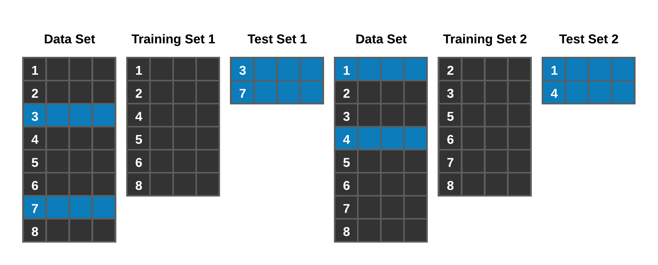
Figure 7.1: The resampling concept

Five-fold cross-validation runs the fit five times and averages the validation metrics (Ian H. Witten 2011). mlr3 makes this easy.

set.seed(44)
resampling <- rsmp("cv", folds = 5)
resampling$instantiate(task_train)

rr <- resample(task_train, learner_rf, resampling, store_models = FALSE)
rr$aggregate(list(
  msr("classif.bacc"),
  msr("classif.auc"),
  msr("classif.prauc")
))

##  classif.bacc   classif.auc classif.prauc 
##     0.5746320     0.6907868     0.3488073

The cross-validated metrics describe expected training-period performance more reliably than one internal split. They do not replace the later evaluation on the future-season holdout.

7.2.1.4.2 Tuning the model

Most algorithms have parameters that change their behavior. A random forest, for instance, can vary the number of candidate variables, trees, terminal-node size, and depth. How do you know you have set them well? You search. We pick a few ranger parameters and a range for each.

tune_space <- ps(
  mtry          = p_int(lower = 2,   upper = length(task_train$feature_names)),
  min.node.size = p_int(lower = 5,   upper = 150),
  max.depth     = p_int(lower = 3,   upper = 20),
  num.trees     = p_int(lower = 300, upper = 800)
)

We need a resampling strategy, a measure, and a stopping rule. We use three-fold cross-validation within the training seasons, optimize ROC AUC because the deliverable is a ranking, and stop after ten evaluations. The future-season test rows still play no role.

# mgcv also exports ti(), so qualify the mlr3tuning constructor.
tune_instance <- mlr3tuning::ti(
  task = task_train,
  learner = learner_rf,
  resampling = rsmp("cv", folds = 3),
  measures = msr("classif.auc"),
  search_space = tune_space,
  terminator = trm("evals", n_evals = 10)
)

A random search samples parameter combinations from those ranges.

set.seed(44)
tuner <- tnr("random_search")
tuner$optimize(tune_instance)

##     mtry min.node.size max.depth num.trees learner_param_vals  x_domain classif.auc
##    <int>         <int>     <int>     <int>             <list>    <list>       <num>
## 1:     4            77         3       335          <list[5]> <list[4]>   0.6940879

The best combination found used 4 candidate variables, a minimum node size of 77, a maximum depth of 3, and 335 trees. Its cross-validated AUC was:

tune_instance$result_y

## classif.auc 
##   0.6940879

We push the winning parameters back into the learner, refit, and predict again.

learner_rf$param_set$values <- tune_instance$result_learner_param_vals
learner_rf$train(task_train)

prediction_tuned <- learner_rf$predict(task_test)
prediction_tuned$confusion

##         truth
## response  nr   r
##       nr  46  11
##       r   87 456

prediction_tuned$score(list(
  msr("classif.acc"),
  msr("classif.bacc"),
  msr("classif.auc"),
  msr("classif.prauc")
))

##   classif.acc  classif.bacc   classif.auc classif.prauc 
##     0.8366667     0.6611550     0.7679155     0.6104686

The tuned model improves every holdout metric: balanced accuracy rises from about 0.622 to 0.661, ROC AUC from 0.721 to 0.768, and precision-recall AUC from 0.539 to 0.610. It also identifies 46 of 133 non-renewers at the default threshold, compared with 35 before tuning. That is a useful but still moderate gain, not a solved retention problem.

7.2.1.5 Comparing different models

Is a random forest the right choice? You only know by trying others. mlr3 makes a fair comparison straightforward through a benchmark: same data, same resampling, several learners. We compare logistic regression, gradient boosting (xgboost), the random forest (ranger), and naive Bayes under the same five-fold splits.

design <- benchmark_grid(
  tasks = task_train,
  learners = list(
    lrn("classif.log_reg", predict_type = "prob"),
    lrn("classif.xgboost", predict_type = "prob"),
    lrn("classif.ranger", predict_type = "prob"),
    lrn("classif.naive_bayes", predict_type = "prob")
  ),
  resamplings = rsmp("cv", folds = 5)
)

set.seed(44)
bmr <- benchmark(design)

We compare them on ROC AUC, precision-recall AUC, and balanced accuracy. Higher is better for all three.

benchmark_measures <- list(
  msr("classif.auc", id = "auc"),
  msr("classif.prauc", id = "prauc"),
  msr("classif.bacc", id = "bacc")
)

bmr$aggregate(benchmark_measures)[, c("learner_id", "auc", "prauc", "bacc")]

##             learner_id       auc     prauc      bacc
##                 <char>     <num>     <num>     <num>
## 1:     classif.log_reg 0.6983282 0.4311043 0.5747098
## 2:     classif.xgboost 0.6402179 0.3141102 0.5568604
## 3:      classif.ranger 0.6838534 0.3715227 0.5867897
## 4: classif.naive_bayes 0.6720478 0.4153668 0.6426478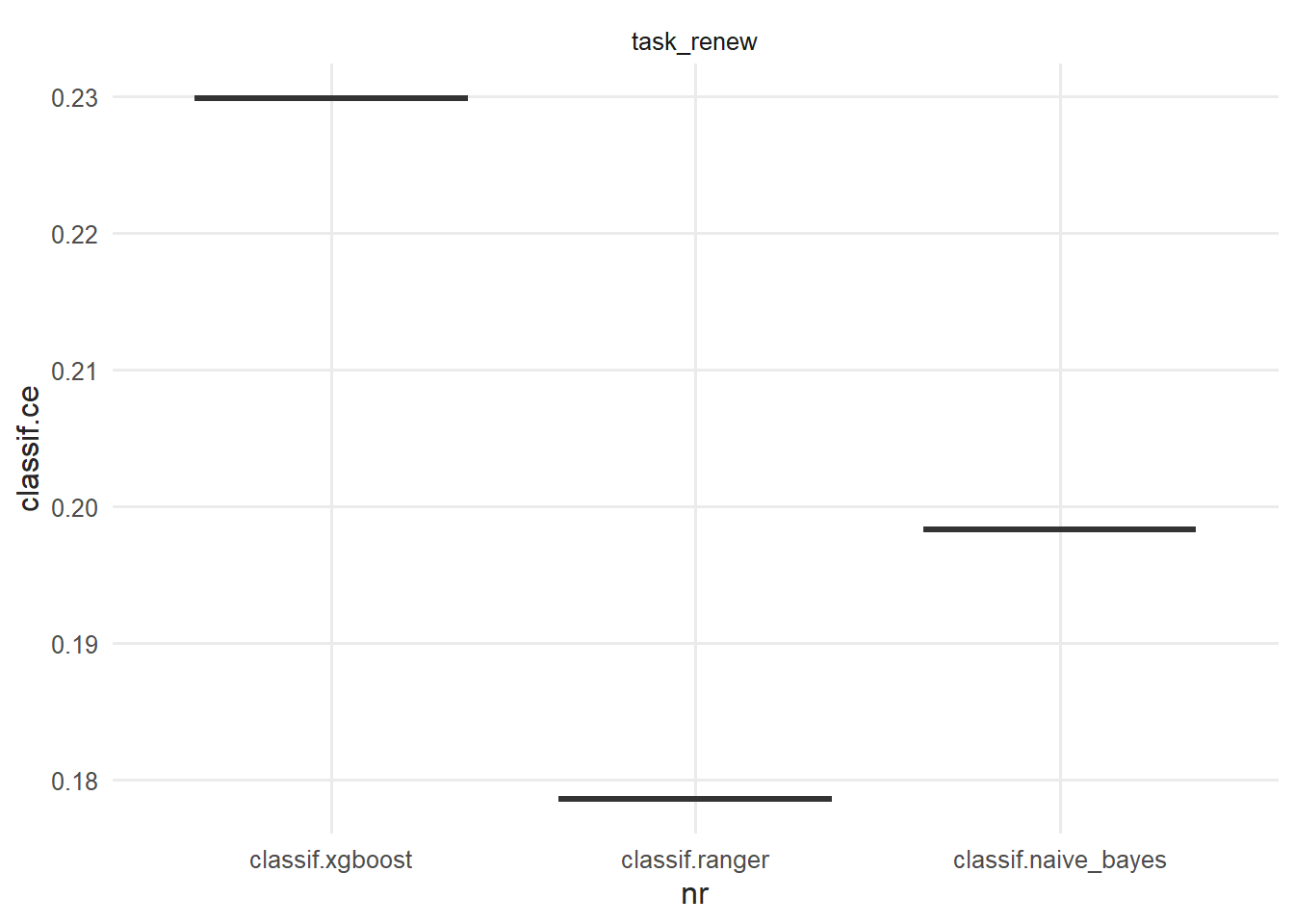

autoplot(bmr, measure = msr("classif.auc")) + book_theme

Figure 7.2: Benchmark ROC AUC by model

Logistic regression has the strongest mean ROC AUC and precision-recall AUC, while naive Bayes has the best balanced accuracy at its default threshold. No learner dominates every measure. That disagreement is useful: model choice must follow the business objective, and threshold tuning is separate from ranking quality. The simpler logistic model is a credible choice here.

7.2.1.6 A logistic regression for comparison

Logistic regression “builds a linear model based on a transformed target variable” (Ian H. Witten 2011). Here it estimates the probability of non-renewal. It is interpretable and a sensible first model for a binary outcome, so it is worth fitting directly.

glm_train <- mod_data_numeric[train_ids, ]
glm_train$renewed <- stats::relevel(glm_train$renewed, ref = "r")

glm_mod <- glm(
  renewed ~ ticketUsage + tenure + spend + distance,
  data = glm_train,
  family = binomial(link = "logit")
)

glm_summary <- tibble::tibble(
  deviance = glm_mod$deviance,
  null_deviance = glm_mod$null.deviance,
  aic = glm_mod$aic,
  pseudo_r2 = 1 - glm_mod$deviance / glm_mod$null.deviance
)

Table 7.6: Logistic regression summary

deviance	null_deviance	aic	pseudo_r2
11236.71	12571.62	11246.71	0.106

The output reads differently from ordinary regression. This direct fit uses four predictors so its coefficients remain readable; the benchmark above is the fair predictive comparison because every learner uses the same feature set and folds. Be careful with the pseudo R-squared because there are several definitions, and it is not a holdout performance metric; pscl::pR2(glm_mod) (Zeileis et al. 2008) shows a few.

7.2.2 Measuring performance

Performance metrics can be technical and confusing. We now use only the untouched 2023 rows to visualize how well the tuned random forest’s non-renewal scores separate the two groups. This keeps the plots honest: training rows would make the model look better than it is.

evaluation_data <- mod_data_numeric[test_ids, ]
evaluation_data$score_churn <- prediction_tuned$prob[, "nr"]

A density plot shows whether renewers and non-renewers receive different churn-risk scores.

ggplot(evaluation_data, aes(x = score_churn, fill = renewed)) +
  geom_density(alpha = 0.4) +
  scale_fill_manual("Outcome", values = plot_palette) +
  scale_x_continuous(labels = scales::percent) +
  labs(x = "Predicted probability of non-renewal", y = "Density",
       title = "The score separates the groups, but they overlap heavily") +
  book_theme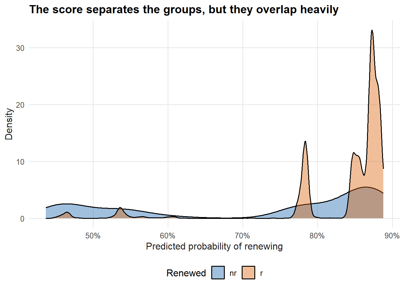

Figure 7.3: Churn-risk density by actual outcome

The distributions shift apart, but they still overlap. An ROC curve summarizes how well the model ranks non-renewers above renewers across every possible threshold.

roc_obj <- pROC::roc(
  evaluation_data$renewed,
  evaluation_data$score_churn,
  levels = c("r", "nr"), direction = "<", quiet = TRUE
)

pROC::ggroc(roc_obj, legacy.axes = TRUE, colour = plot_palette[1], linewidth = 1.2) +
  geom_abline(slope = 1, intercept = 0, linetype = 2, color = "grey50") +
  labs(x = "False-positive rate", y = "True-positive rate for non-renewal",
       title = paste0("Holdout AUC = ", round(as.numeric(roc_obj$auc), 3))) +
  book_theme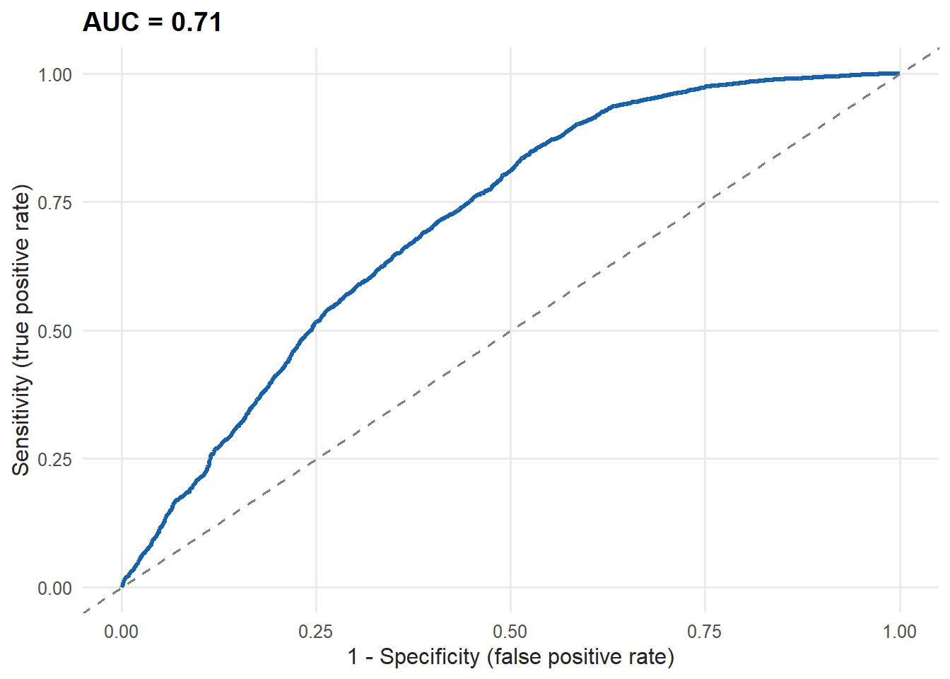

Figure 7.4: ROC curve for the non-renewal model

The dashed diagonal is what random guessing would produce. Our curve sits above it, so the model has real, if limited, discriminatory power. AUC measures ranking, not probability calibration. If a workflow uses a score such as 0.70 as a literal 70% risk, check calibration and a proper scoring rule such as the Brier score before deployment.

7.3 Using the model

A churn score can also reproduce inequities embedded in historical service, pricing, geography, or access. Before deployment, inspect performance and contact rates across relevant groups, exclude fields that are not appropriate for the decision, document overrides, and give account representatives a way to report systematic errors.

Lead scores are easy to calculate, but operational deployment still requires careful integration. Qualifying leads may nevertheless be one of the highest-value analytics tasks a club can deploy quickly. You apply the model to current accounts, sort by the score, and work the list in whatever order serves the goal. Because the score now measures non-renewal directly, the manager works from the top: highest churn risk first. After evaluation, refit the chosen specification on all available history before scoring a genuinely future cohort.

7.3.1 Cumulative gains charts

How much does the model actually help in practice? A cumulative gains chart answers that. Sort the holdout accounts by churn risk, then ask: if we work the top X% of the list, what share of all non-renewers have we reached? A model with no skill captures non-renewers at the same rate as the population, which produces the diagonal. A useful model bows above it.

gains <- evaluation_data |>
  dplyr::select(renewed, score_churn) |>
  dplyr::arrange(desc(score_churn)) |>
  dplyr::mutate(
    churn_flag = as.integer(renewed == "nr"),
    population_pct = row_number() / n(),
    captured_pct = cumsum(churn_flag) / sum(churn_flag)
  )

ggplot(gains, aes(x = population_pct, y = captured_pct)) +
  geom_line(color = plot_palette[1], linewidth = 1.2) +
  geom_abline(slope = 1, intercept = 0, linetype = 2, color = "grey50") +
  scale_x_continuous(labels = scales::percent) +
  scale_y_continuous(labels = scales::percent) +
  labs(x = "Share of accounts worked", y = "Share of non-renewers captured",
       title = "Working highest-risk accounts first finds churn sooner") +
  book_theme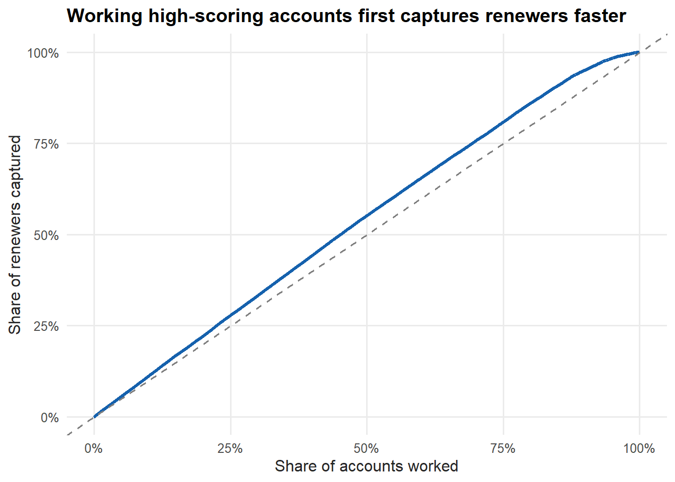

Figure 7.5: Cumulative gains chart

The curve sits above the diagonal, so prioritizing high-scoring accounts does find non-renewers faster than working the list at random, but the gap is modest, consistent with the model’s limited discrimination. The further the curve bows toward the top-left corner, the more your campaign benefits from the scoring. Where the curve flattens, additional outreach is buying you little, which is a natural place to stop a campaign.

7.4 Key concepts and chapter summary

Systematically prioritizing whom to contact is core to direct marketing. We covered:

• RFM scores
• Lead scoring with a random forest in mlr3
• Cross-validation
• Model tuning
• Model comparison via benchmarking
• Evaluating a model with confusion matrices, ROC, and gains charts
• Putting the scores to work

A few lessons are worth keeping:

• RFM scoring is simple, interpretable, and a fine starting point, sometimes called the “poor analyst’s analytics.”
• A random forest is a strong predictive default for many tabular club data sets, but it is less interpretable than logistic regression.
• Mind the base rate. With 81% of accounts renewing, accuracy is a misleading headline. Judge a model by how well it finds the minority you care about, using the confusion matrix, balanced accuracy, ROC AUC, precision-recall AUC, and business costs.
• Cross-validate and tune, but stay honest about how much they actually buy you.
• Compare several models. They often finish close together, and the ranking can change across folds and seeds, which is reason enough to prefer the simpler one when performance is materially equivalent.
• Deployment is an operational system, not a spreadsheet handoff. Integrate scores into the CRM, define ownership and capacity, capture outcomes, monitor drift and group-level performance, and retrain only when validation supports it.

Chapter 8 turns to promotions, including designing offers and, harder still, figuring out whether they actually caused the sales we attribute to them.